PI control

In this tutorial we’ll introduce

1. PI control, a commonly used model-free control method,

2. how to estimate the firing rate using a causal, exponential filter, and

3. modeling computation delays to reflect hardware and algorithmic speed limitations present in a real experiment.

Imports, etc.:

import brian2.only as b2
from brian2 import np, ms
import matplotlib.pyplot as plt
import cleo

cleo.utilities.style_plots_for_docs()

np.random.seed(18990508)
b2.seed(19920323)

# the default cython compilation target isn't worth it for this trivial example
b2.prefs.codegen.target = "numpy"

# colors
c = {
    "light": "#df87e1",
    "main": "#C500CC",
    "dark": "#8000B4",
    "accent": "#36827F",
    "accent_light": "#69fff8",
}

Create the Brian network

We’ll create a population of 10 LIF neurons mainly driven by feedforward input but with some recurrent connections as well.

n = 10
population = b2.NeuronGroup(
    n,
    """
    dv/dt = (-v - 70*mV + Rm*I) / tau : volt
    tau: second
    Rm: ohm
    I: amp""",
    threshold="v>-50*mV",
    reset="v=-70*mV",
)
population.tau = 10 * ms
population.Rm = 100 * b2.Mohm
population.I = 0 * b2.mA
population.v = -70 * b2.mV

input_group = b2.PoissonGroup(n, np.linspace(20, 200, n) * b2.Hz)

S = b2.Synapses(input_group, population, on_pre="v+=5*mV")
S.connect(condition=f"abs(i-j)<={3}")
S2 = b2.Synapses(population, population, on_pre="v+=2*mV")
S2.connect(p=0.2)

pop_mon = b2.SpikeMonitor(population)

net = b2.Network(population, input_group, S, S2, pop_mon)
population.equations

\[\begin{split}\begin{align*}\frac{\mathrm{d}v}{\mathrm{d}t} &= \frac{I Rm - 70 mV - v}{\tau} && \text{(unit of $v$: $\mathrm{V}$)}\\ I &&& \text{(unit: $\mathrm{A}$)}\\ Rm &&& \text{(unit: $\mathrm{ohm}$)}\\ \tau &&& \text{(unit: $\mathrm{s}$)}\end{align*}\end{split}\]

Run simulation without control:

net.run(100 * b2.ms)

INFO       No numerical integration method specified for group 'neurongroup', using method 'exact' (took 0.63s). [brian2.stateupdaters.base.method_choice]

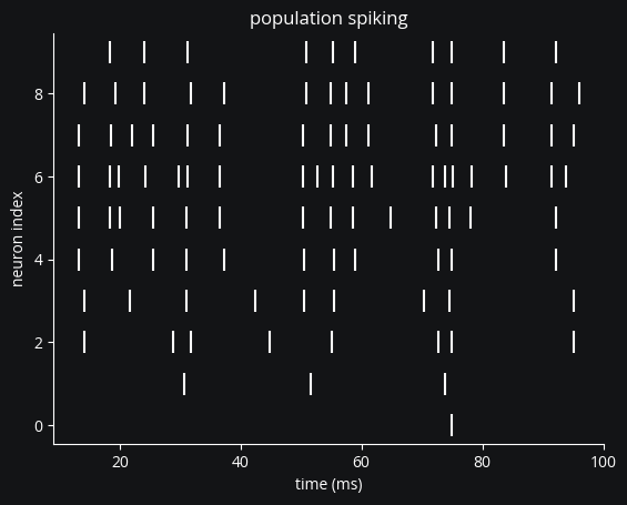
fig, ax = plt.subplots()
ax.scatter(pop_mon.t / ms, pop_mon.i, marker="|", c="w", s=200)
ax.set(title="population spiking", ylabel="neuron index", xlabel="time (ms)");

Constructing a closed-loop simulation

We will use the popular model-free PI control to control a single neuron’s firing rate. PI stands for proportional-integral, referring to a feedback gain proportional to the instantaneous error as well as the integrated error over time.

First we construct a CLSimulator from the network:

sim = cleo.CLSimulator(net)

Then, to control neuron \(i\), we need to:

1. capture spiking using a GroundTruthSpikeRecorder

i = 0  # neuron to control
rec = cleo.recorders.GroundTruthSpikeRecorder(name="spike_rec")
sim.inject(rec, population[i])

CLSimulator(io_processor=None, devices={GroundTruthSpikeRecorder(name='spike_rec', save_history=True, _mon=<SpikeMonitor, recording from 'spikemonitor_1'>, _num_spikes_seen=0, neuron_group=<Subgroup 'neurongroup_subgroup' of 'neurongroup' from 0 to 1>)})

2. define the firing rate trajectory we want our target neuron to follow

# the target firing rate trajectory, as a function of time
def target(t):
    a = 200
    sinusoid = a + a * np.sin(2 * np.pi * 20 * b2.Hz * t)
    out_Hz = 400 * (t < 250 * ms) + sinusoid * (t >= 250 * ms)
    return np.squeeze(out_Hz) * b2.Hz

2. estimating its firing rate from incoming spikes using exp_firing_rate_estimate()

3. compute the stimulus intensity with pi_ctrl()

4. output that value for a StateVariableSetter stimulator to use

Here we initialize needed variables when the IOProcessor is created and define how to process network output and set the control signal in the process() function. The reset() function is called automatically on cleo.CLSimulator.reset() and should be used to re-initialize variables as needed.

from cleo.ioproc import LatencyIOProcessor, exp_firing_rate_estimate, pi_ctrl


class PIRateIOProcessor(LatencyIOProcessor):
    def __init__(self):
        super().__init__(sample_period=1 * ms)
        # for firing rate estimation
        self.fr_est_tau = 15 * ms

        # error will be in frequency units (firing rate)
        self.Kp = 0.005 / b2.Hz
        # integral error will have no unit (frequency times time)
        self.Ki = 0.04 / (b2.Hz * b2.second)

        self.delay = 7 * ms

        # initializes variables
        self.reset()

    def process(self, state_dict, t_samp):
        spikes = state_dict["spike_rec"]
        prev_rate = self.fr_estimates[-1] if len(self.fr_estimates) > 0 else 0
        fr = exp_firing_rate_estimate(
            spikes, self.sample_period, prev_rate, self.fr_est_tau
        )
        self.fr_estimates.append(fr)

        ctrl_signal, self.int_error = pi_ctrl(
            measurement=fr,
            reference=target(t_samp),
            integ_error=self.int_error,
            dt=self.sample_period,
            Kp=self.Kp,
            Ki=self.Ki,
        )

        # this dictionary output format allows for the flexibility
        # of controlling multiple stimulators
        # limit to positive current
        ctrl_signal = ctrl_signal * (ctrl_signal > 0)
        # grab just first element from 1-length sequence
        # since StateVariableSetter only takes a scalar
        ctrl_signal = ctrl_signal[0]
        out_dict = {"I_stim": ctrl_signal}

        # simulate delayed control by adding to the output time
        out_time = t_samp + self.delay
        return out_dict, out_time

    def reset(self):
        self.fr_estimates = []
        self.int_error = 0


io_processor = PIRateIOProcessor()
sim.set_io_processor(io_processor)

CLSimulator(io_processor=PIRateIOProcessor(sample_period=1. * msecond, sampling='fixed', processing='parallel'), devices={GroundTruthSpikeRecorder(name='spike_rec', save_history=True, _mon=<SpikeMonitor, recording from 'spikemonitor_1'>, _num_spikes_seen=0, neuron_group=<Subgroup 'neurongroup_subgroup' of 'neurongroup' from 0 to 1>)})

Here we simply added a constant delay at the end, but in a complex, multi-step computation, we could add a probabilistic delay for each step to better approximate a real-world latency distribution.

Now we inject the stimulator:

stim = cleo.stimulators.StateVariableSetter(
    name="I_stim", variable_to_ctrl="I", unit=b2.nA
)
sim.inject(stim, population[i])

CLSimulator(io_processor=PIRateIOProcessor(sample_period=1. * msecond, sampling='fixed', processing='parallel'), devices={GroundTruthSpikeRecorder(name='spike_rec', save_history=True, _mon=<SpikeMonitor, recording from 'spikemonitor_1'>, _num_spikes_seen=0, neuron_group=<Subgroup 'neurongroup_subgroup' of 'neurongroup' from 0 to 1>), StateVariableSetter(name='I_stim', save_history=True, value=0, variable_to_ctrl='I', unit=namp, neuron_groups=[<Subgroup 'neurongroup_subgroup_1' of 'neurongroup' from 0 to 1>])})

Run the simulation

sim.run(300 * ms)

def plot_results():
    fig, (ax1, ax2, ax3) = plt.subplots(3, 1, sharex=True, layout="compressed")
    ax1.plot(pop_mon.t / ms, pop_mon.i, "|", c="w")
    ax1.plot(
        pop_mon.t[pop_mon.i == i] / ms,
        pop_mon.i[pop_mon.i == i],
        "|",
        c=c["main"],
    )
    ax1.set(title="population spiking", ylabel="neuron index")

    ax2.plot(
        io_processor.t_samp / ms,
        io_processor.fr_estimates,
        c=c["main"],
    )
    ax2.plot(
        io_processor.t_samp / ms,
        target(io_processor.t_samp),
        c="xkcd:fluorescent green",
        linestyle="--",
    )

    ax2.set(ylabel="firing rate (Hz)", title=f"neuron {i} activity")
    ax2.legend(["estimated firing rate", "target firing rate"])
    ax3.plot(
        stim.t / ms,
        stim.values,
        c=c["accent_light"],
    )
    ax3.set(title="control input", ylabel="$I_{stim}$ (nA)", xlabel="time (ms)")


plot_results()

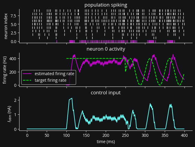
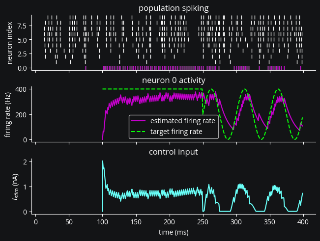
Note the lag in keeping up with the target firing rate, which can be directly attributed to the ~7 ms delay we coded in to the IO processor. Let’s compare to the result with a short delay. We can use reset() to reset the simulation back to the last time we changed it (in this case when we injected the stimulator).

sim.reset()
io_processor.delay = 0.1 * ms
sim.run(300 * ms)
plot_results()

Conclusion

In this tutorial, we’ve learned how to

• use pi_ctrl() to interact with a Brian simulation,

• estimate firing rate with exp_firing_rate_estimate(), and

• introduce delay to the control output to model real-life latency.