Advanced LFP#
Here we will demonstrate the diverse ways the different LFP proxies can be computed and compare them to each other.
# preamble:
import brian2.only as b2
from brian2 import np
import matplotlib.pyplot as plt
import cleo
from cleo import ephys
import cleo.utilities

# the default cython compilation target isn't worth it for
# this trivial example
b2.prefs.codegen.target = "numpy"
b2.seed(18010601)
np.random.seed(18010601)
rng = np.random.default_rng(18010601)

cleo.utilities.style_plots_for_docs()

# colors
c = {
    "light": "#df87e1",
    "main": "#C500CC",
    "dark": "#8000B4",
    "exc": "#d6755e",
    "inh": "#056eee",
    "accent": "#36827F",
}
Network setup#
First we need a point neuron simulation to approximate the LFP for. Here we adapt a balanced E/I network implementation from the Neuronal Dynamics textbook, using some parameters from Mazzoni, Lindén et al., 2015.
n_exc = 800
n_inh = None  # None = N_excit / 4
n_ext = 100
connection_probability = 0.2
w0 = 0.07 * b2.nA
g = 4
synaptic_delay = 1 * b2.ms
poisson_input_rate = 220 * b2.Hz
w_ext = 0.091 * b2.nA
v_rest = -70 * b2.mV
v_reset = -60 * b2.mV
firing_threshold = -50 * b2.mV
membrane_time_scale = 20 * b2.ms
Rm = 100 * b2.Mohm
abs_refractory_period = 2 * b2.ms

if n_inh is None:
    n_inh = int(n_exc / 4)
N_tot = n_exc + n_inh
if n_ext is None:
    n_ext = int(n_exc * connection_probability)
if w_ext is None:
    w_ext = w0

J_excit = w0
J_inhib = -g * w0

lif_dynamics = """
    dv/dt = (-(v-v_rest) + Rm*(I_exc + I_ext + I_gaba)) / membrane_time_scale : volt (unless refractory)
    I_gaba : amp
    I_exc : amp
    I_ext : amp
"""

neurons = b2.NeuronGroup(
    N_tot,
    model=lif_dynamics,
    threshold="v>firing_threshold",
    reset="v=v_reset",
    refractory=abs_refractory_period,
    method="linear",
)
neurons.v = (
    np.random.uniform(
        v_rest / b2.mV, high=firing_threshold / b2.mV, size=(n_exc + n_inh)
    )
    * b2.mV
)
cleo.coords.assign_coords_rand_cylinder(
    neurons, (0, 0, 700), (0, 0, 900), 250, unit=b2.um
)

exc = neurons[:n_exc]
inh = neurons[n_exc:]

syn_eqs = """
    dI_syn_syn/dt = (s - I_syn_syn)/tau_dsyn : amp (clock-driven)
    I_TYPE_post = I_syn_syn : amp (summed)
    ds/dt = -s/tau_rsyn : amp (clock-driven)
"""

exc_synapses = b2.Synapses(
    exc,
    target=neurons,
    model=syn_eqs.replace("TYPE", "exc"),
    on_pre="s += J_excit",
    delay=synaptic_delay,
    namespace={"tau_rsyn": 0.4 * b2.ms, "tau_dsyn": 2 * b2.ms},
)
exc_synapses.connect(p=connection_probability)

inh_synapses = b2.Synapses(
    inh,
    target=neurons,
    model=syn_eqs.replace("TYPE", "gaba"),
    on_pre="s += J_inhib",
    delay=synaptic_delay,
    namespace={"tau_rsyn": 0.25 * b2.ms, "tau_dsyn": 5 * b2.ms},
)
inh_synapses.connect(p=connection_probability)

ext_input = b2.PoissonGroup(n_ext, poisson_input_rate, name="ext_input")
ext_synapses = b2.Synapses(
    ext_input,
    target=neurons,
    model=syn_eqs.replace("TYPE", "ext"),
    on_pre="s += w_ext",
    delay=synaptic_delay,
    namespace={"tau_rsyn": 0.4 * b2.ms, "tau_dsyn": 2 * b2.ms},
)
ext_synapses.connect(p=connection_probability)

net = b2.Network(
    neurons,
    exc_synapses,
    inh_synapses,
    ext_input,
    ext_synapses,
)
sim = cleo.CLSimulator(net)
Electrode setup#
elec_coords = cleo.ephys.linear_shank_coords(1 * b2.mm, channel_count=10)
elec_coords = cleo.ephys.tile_coords(
    elec_coords, num_tiles=3, tile_vector=(500, 0, 0) * b2.um
)
probe = cleo.ephys.Probe(elec_coords)
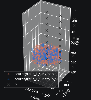
cleo.viz.plot(
    exc,
    inh,
    colors=[c["exc"], c["inh"]],
    zlim=(0, 1200),
    devices=[probe],
    scatterargs={"alpha": 0.3},
);
mua = ephys.MultiUnitSpiking(
    r_perfect_detection=0.05 * b2.mm,
    r_half_detection=0.1 * b2.mm,
)
ss = ephys.SortedSpiking(0.05 * b2.mm, 0.1 * b2.mm)
tklfp = ephys.TKLFPSignal()
RWSLFP recording options#
There are a few important variations on how to record RWSLFP:
Currents can be summed over the population, so that a postsynaptic current (PSC) in one location has the same effect on LFP as one on the other side of the population. The main advantage to this approach is it saves some memory storing currents. To use this, set
pop_aggregatetoTrue. You’ll also want to setamp_functowslfp.mazzoni15_popto get the population amplitude profile from Mazzoni et al., 2015. The default is to not sum over the population, and usewslfp.mazzoni15_nrnto get per-neuron contributions to LFP instead.The LFP can be computed from PSCs if your model simulates them or from spikes (after synthesizing PSCs from them). Use
RWSLFPSignalFromSpikesorRWSLFPSignalFromPSCsaccordingly. In this example, we are simulating synaptic dynamics in the form of biexponential currents, which happens to be the form used to generate synthetic PSCs.
RWSLFPSignalFromSpikes needs to know about all spikes transmitted to the population being recorded from, so ampa_syns and gaba_syns must be passed on injection.
To account for the relative impact of incoming spikes on synaptic currents, Cleo needs to be able to find the weight as well.
It looks for a variable or parameter named w in the synapses by default, but you can pass in an alternate name or a value on injection instead.
RWSLFPSignalFromSpikes has sensible defaults, but can be overridden with the exact parameters used in our model.
These are used in the synthetic current generation process.
These parameters then serve as the default for the signal, which can be overridden on a per-injection basis.
import wslfp

rwslfp_spk_nrn = ephys.RWSLFPSignalFromSpikes(
    tau1_ampa=exc_synapses.namespace["tau_dsyn"],
    tau2_ampa=exc_synapses.namespace["tau_rsyn"],
    tau1_gaba=inh_synapses.namespace["tau_dsyn"],
    tau2_gaba=inh_synapses.namespace["tau_rsyn"],
    syn_delay=synaptic_delay,
    name="per-neuron RWSLFP from spikes",
)

rwslfp_spk_pop = ephys.RWSLFPSignalFromSpikes(
    pop_aggregate=True,
    amp_func=wslfp.mazzoni15_pop,
    name="population-aggregated RWSLFP from spikes",
)
All that’s needed for RWSLFPSignalFromPSCs is Iampa_var_names and Igaba_var_names on injection, which are lists of the variables representing AMPA and GABA currents.
rwslfp_psc_nrn = ephys.RWSLFPSignalFromPSCs(name="per-neuron RWSLFP from PSCs")
rwslfp_psc_pop = ephys.RWSLFPSignalFromPSCs(
    pop_aggregate=True,
    amp_func=wslfp.mazzoni15_pop,
    name="population-aggregated RWSLFP from PSCs",
)
All signals are grouped together on the probe, but we can avoid RWSLFP being recorded from interneurons by omitting ampa_syns, gaba_syns, Iampa_var_names, and Igaba_var_names from the injection.
probe.add_signals(
    mua,
    ss,
    tklfp,
    rwslfp_spk_nrn,
    rwslfp_spk_pop,
    rwslfp_psc_nrn,
    rwslfp_psc_pop,
)

sim.set_io_processor(cleo.ioproc.RecordOnlyProcessor(sample_period_ms=1))
sim.inject(
    probe,
    exc,
    # for TKLFPSignal:
    tklfp_type="exc",
    # for RWSLFPSignalFromSpikes:
    synaptic_delay=synaptic_delay,  # can override for all synapses
    ampa_syns=[  # or per synapse by with (syn, kwargs) tuples:
        # want only synapses onto pyramidal cells
        (exc_synapses[f"j < {n_exc}"], {"weight": J_excit}),
        (ext_synapses[f"j < {n_exc}"], {"weight": w_ext}),
    ],
    gaba_syns=[(inh_synapses[f"j < {n_exc}"], {"weight": J_inhib})],
    # for RWSLFPSignalFromPSCs:
    Iampa_var_names=["I_exc", "I_ext"],
    Igaba_var_names=["I_gaba"],
)
# we don't include ampa_syns, gaba_syns, Iampa_var_name, or Igaba_var_name since RWSLFP
# is only recorded from pyramidal cells
sim.inject(probe, inh, tklfp_type="inh")
---------------------------------------------------------------------------
DimensionMismatchError                    Traceback (most recent call last)
Cell In[17], line 12
      1 probe.add_signals(
      2     mua,
      3     ss,
   (...)
      8     rwslfp_psc_pop,
      9 )
     11 sim.set_io_processor(cleo.ioproc.RecordOnlyProcessor(sample_period_ms=1))
---> 12 sim.inject(
     13     probe,
     14     exc,
     15     # for TKLFPSignal:
     16     tklfp_type="exc",
     17     # for RWSLFPSignalFromSpikes:
     18     synaptic_delay=synaptic_delay,  # can override for all synapses
     19     ampa_syns=[  # or per synapse by with (syn, kwargs) tuples:
     20         # want only synapses onto pyramidal cells
     21         (exc_synapses[f"j < {n_exc}"], {"weight": J_excit}),
     22         (ext_synapses[f"j < {n_exc}"], {"weight": w_ext}),
     23     ],
     24     gaba_syns=[(inh_synapses[f"j < {n_exc}"], {"weight": J_inhib})],
     25     # for RWSLFPSignalFromPSCs:
     26     Iampa_var_names=["I_exc", "I_ext"],
     27     Igaba_var_names=["I_gaba"],
     28 )
     29 # we don't include ampa_syns, gaba_syns, Iampa_var_name, or Igaba_var_name since RWSLFP
     30 # is only recorded from pyramidal cells
     31 sim.inject(probe, inh, tklfp_type="inh")

File ~/miniforge3/lib/python3.10/site-packages/cleo/base.py:383, in CLSimulator.inject(self, device, *neuron_groups, **kwparams)
    381         device.sim = self
    382         device.init_for_simulator(self)
--> 383     device.connect_to_neuron_group(ng, **kwparams)
    384 for brian_object in device.brian_objects:
    385     if brian_object not in self.network.objects:

File ~/miniforge3/lib/python3.10/site-packages/cleo/ephys/probes.py:158, in Probe.connect_to_neuron_group(self, neuron_group, **kwparams)
    146 """Configure probe to record from given neuron group
    147
    148 Will call :meth:`Signal.connect_to_neuron_group` for each signal
   (...)
    155     Passed in to signals' connect functions, needed for some signals
    156 """
    157 for signal in self.signals:
--> 158     signal.connect_to_neuron_group(neuron_group, **kwparams)
    159     self.brian_objects.update(signal.brian_objects)

File ~/miniforge3/lib/python3.10/site-packages/cleo/ephys/spiking.py:209, in MultiUnitSpiking.connect_to_neuron_group(self, neuron_group, **kwparams)
    201 def connect_to_neuron_group(self, neuron_group: NeuronGroup, **kwparams) -> None:
    202     """Configure signal to record from specified neuron group
    203
    204     Parameters
   (...)
    207         group to record from
    208     """
--> 209     neuron_channel_dtct_probs = super(
    210         MultiUnitSpiking, self
    211     ).connect_to_neuron_group(neuron_group, **kwparams)
    212     if self._dtct_prob_array is None:
    213         self._dtct_prob_array = neuron_channel_dtct_probs

File ~/miniforge3/lib/python3.10/site-packages/cleo/ephys/spiking.py:100, in Spiking.connect_to_neuron_group(self, neuron_group, **kwparams)
     98 distances = np.sqrt(dist2) * meter  # since units stripped
     99 # probs is n_neurons by n_channels
--> 100 probs = self._detection_prob_for_distance(distances)
    101 # cut off to get indices of neurons to monitor
    102 # [0] since nonzero returns tuple of array per axis
    103 i_ng_to_keep = np.nonzero(np.all(probs > self.cutoff_probability, axis=1))[0]

File ~/miniforge3/lib/python3.10/site-packages/cleo/ephys/spiking.py:149, in Spiking._detection_prob_for_distance(self, r)
    147 h = b - a
    148 with np.errstate(divide="ignore"):
--> 149     decaying_p = h / (r - c)
    150 decaying_p[decaying_p == np.inf] = 1  # to fix NaNs caused by /0
    151 p = 1 * (r <= a) + decaying_p * (r > a)

File ~/miniforge3/lib/python3.10/site-packages/brian2/units/fundamentalunits.py:1193, in Quantity.__array_ufunc__(self, uf, method, *inputs, **kwargs)
   1190 elif uf.__name__ in UFUNCS_MATCHING_DIMENSIONS + UFUNCS_COMPARISONS:
   1191     # Ok if dimension of arguments match (for reductions, they always do)
   1192     if method == "__call__":
-> 1193         fail_for_dimension_mismatch(
   1194             inputs[0],
   1195             inputs[1],
   1196             error_message=(
   1197                 "Cannot calculate {val1} %s {val2}, the units do not match"
   1198             )
   1199             % uf.__name__,
   1200             val1=inputs[0],
   1201             val2=inputs[1],
   1202         )
   1203     if uf.__name__ in UFUNCS_COMPARISONS:
   1204         return uf_method(*[np.asarray(i) for i in inputs], **kwargs)

File ~/miniforge3/lib/python3.10/site-packages/brian2/units/fundamentalunits.py:266, in fail_for_dimension_mismatch(obj1, obj2, error_message, **error_quantities)
    264         raise DimensionMismatchError(error_message, dim1)
    265     else:
--> 266         raise DimensionMismatchError(error_message, dim1, dim2)
    267 else:
    268     return dim1, dim2

DimensionMismatchError: Cannot calculate [[744.49268121 633.67308509 ... 493.58269913 537.05397445]
 [738.41717567 633.80230596 ... 751.65265837 786.73885169]
 ...
 [855.56910977 748.6961901  ... 719.53451027 737.43356252]
 [878.30703686 769.1187142  ... 650.4913611  663.92034206]] mm^2 subtract 0. m, the units do not match (units are m^2 and m).
Run simulation and plot results#
sim.reset()
sim.run(500 * b2.ms)
INFO       No numerical integration method specified for group 'synapses_1', using method 'exact' (took 0.29s). [brian2.stateupdaters.base.method_choice]
INFO       No numerical integration method specified for group 'synapses_2', using method 'exact' (took 0.16s). [brian2.stateupdaters.base.method_choice]
INFO       No numerical integration method specified for group 'synapses', using method 'exact' (took 0.00s). [brian2.stateupdaters.base.method_choice]
from matplotlib.colors import ListedColormap
fig, axs = plt.subplots(2, 1, sharex=True)
# assuming all neurons are detectable for c=ss.i >= n_e to work
# in practice this will often not be the case and we'd have to map
# from probe index to neuron group index using ss.i_probe_by_i_ng.inverse
exc_inh_cmap = ListedColormap([c["exc"], c["inh"]])
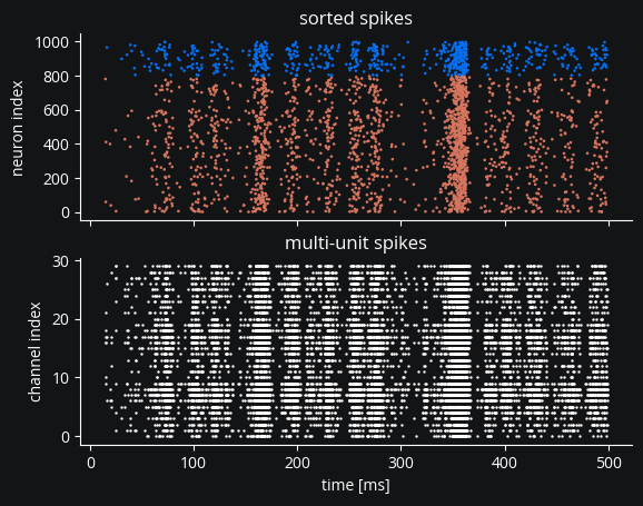
axs[0].scatter(ss.t_ms, ss.i, marker=".", c=ss.i >= n_exc, cmap=exc_inh_cmap, s=3)
axs[0].set(title="sorted spikes", ylabel="neuron index")
axs[1].scatter(mua.t_ms, mua.i, marker=".", s=2, c="white")
axs[1].set(title="multi-unit spikes", ylabel="channel index", xlabel="time [ms]");
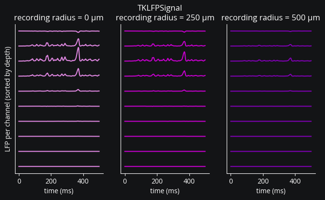
def plot_lfp(t_ms, lfp, title=None):
    n_shanks = 3
    n_contacts_per_shank = 10
    fig, axs = plt.subplots(1, n_shanks, sharey=True, figsize=(8, 4))
    for i, color, r_rec, ax in zip(
        range(n_shanks), [c["light"], c["main"], c["dark"]], [0, 250, 500], axs
    ):
        lfp_for_shank = lfp[
            :, i * n_contacts_per_shank : (i + 1) * n_contacts_per_shank
        ]
        ax.plot(
            t_ms,
            lfp_for_shank + np.arange(n_contacts_per_shank) * 1.1 * np.abs(lfp.max()),
            c=color,
        )
        ax.set(xlabel="time (ms)", yticks=[], title=f"recording radius = {r_rec} µm")

    axs[0].set(ylabel="LFP per channel (sorted by depth)")
    if title:
        fig.suptitle(title)


for signal in probe.signals:
    if isinstance(
        signal,
        (ephys.TKLFPSignal, ephys.RWSLFPSignalFromPSCs, ephys.RWSLFPSignalFromSpikes),
    ):
        lfp = signal.lfp
    else:
        continue
    plot_lfp(signal.t_ms, lfp, title=signal.name)
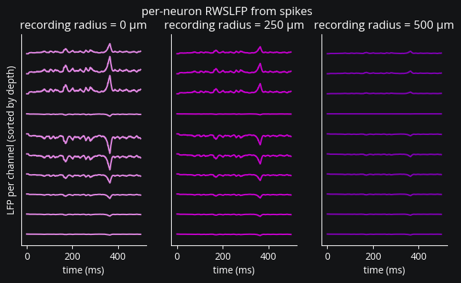
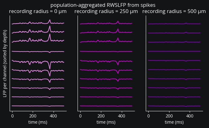
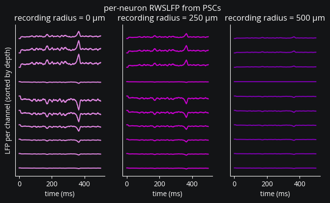
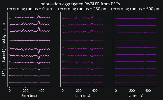
Despite using all the same parameters for the postsynaptic current curves, the FromSpikes and FromPSCs signals look different.
In fact, what we see above matches the WSLFP demo, where the spike convolution signal is somewhat spikier (i.e., with higher peaks the jump at the beginning looks smaller).