LQR optimal control using ldsctrlest

This tutorial will be more comprehensive than the others, bringing together all of cleo’s main capabilities—electrode recording, optogenetics, and latency modeling—as well as introducing more sophisticated model-based feedback control. To achieve the latter, we will use the Python bindings to the ldsCtrlEst C++ library.

First some boilerplate:

from brian2 import ms, mm, um, second, mV, Hz, np
import brian2.only as b2
import matplotlib.pyplot as plt
import cleo

cleo.utilities.style_plots_for_docs()

# numpy faster than cython for lightweight example
b2.prefs.codegen.target = "numpy"
np.random.seed(17320222)
b2.seed(17870917)
cleo.utilities.set_seed(17991214)

cy1 = "#C500CC"
cy2 = "#df87e1"
cu1 = cleo.utilities.wavelength_to_rgb(463 * b2.nmeter)
cu2 = cleo.utilities.wavelength_to_rgb(483 * b2.nmeter)

Network setup

For the network model we adapt an E/I network implementation from the Neuronal Dynamics textbook. Let’s run it and plot the spiking output:

Show code cell source Hide code cell source

b2.defaultclock.dt = 0.5 * b2.ms

n_exc = 80
n_inh = int(n_exc / 4)
connection_probability = 0.1
n_ext = int(n_exc * connection_probability)
w0 = 0.1 * b2.mV  # 0.2
g = 4
w_inh = -g * w0
synaptic_delay = 1.5 * b2.ms
w_external = w0
v_rest = -70 * b2.mV
v_reset = -60 * b2.mV
firing_threshold = -50 * b2.mV
tau_m = 20 * b2.ms
Rm = 100 * b2.Mohm
abs_refractory_period = 2 * b2.ms
thresh_rate = (firing_threshold - v_rest) / (w_external * n_ext * tau_m)
poisson_input_rate = 1 * thresh_rate
bias_current = 11 * b2.pA
# I_bias = b2.TimedArray((np.arange(20) % 2 == 0) * bias_current, dt=100 * b2.ms)

bias_ng = b2.NeuronGroup(
    1, "dI_bias/dt = -I_bias / second + bias_current*xi/sqrt(tau_m) : amp"
)

lif_dynamics = """
dv/dt = (-(v-v_rest) + Rm * (I + I_bias)) / tau_m : volt (unless refractory)
I : amp
I_bias : amp (linked)
"""

ng = b2.NeuronGroup(
    n_exc + n_inh,
    model=lif_dynamics,
    threshold="v>firing_threshold",
    reset="v=v_reset",
    refractory=abs_refractory_period,
    method="linear",
)
ng.I_bias = b2.linked_var(bias_ng, "I_bias")

# random v init
ng.v = (
    np.random.uniform(
        v_rest / b2.mV, high=firing_threshold / b2.mV, size=(n_exc + n_inh)
    )
    * b2.mV
)
ng_exc = ng[:n_exc]
ng_inh = ng[n_exc:]

syn = b2.Synapses(
    ng,
    model="w : volt",
    on_pre="v += w",
    delay=synaptic_delay,
)
syn.connect(p=connection_probability)
syn[f"i < {n_exc}"].w = w0
syn[f"i >= {n_exc}"].w = w_inh

external_poisson_input = b2.PoissonInput(
    target=ng,
    target_var="v",
    N=n_ext,
    rate=poisson_input_rate,
    weight=w_external,
)

rate_monitor = b2.PopulationRateMonitor(ng)
spike_monitor = b2.SpikeMonitor(ng, record=True)
# voltage_monitor = b2.StateMonitor(neurons, "v", record=idx_monitored_neurons)

net = b2.Network(
    ng,
    bias_ng,
    syn,
    external_poisson_input,
    rate_monitor,
    spike_monitor,
    # voltage_monitor,
)

runtime = 1 * b2.second
net.store()
net.run(runtime)

plt.scatter(spike_monitor.t / b2.ms, spike_monitor.i, s=1)
net.restore()

INFO       No numerical integration method specified for group 'neurongroup', using method 'euler' (took 0.02s, trying other methods took 0.00s). [brian2.stateupdaters.base.method_choice]

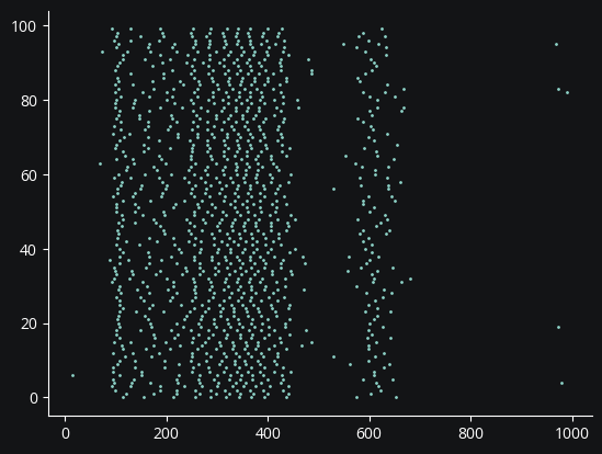
The spiking looks like we want: relatively stable with random fluctuations in global activity from the bias current we added. This will make things more interesting for the controller.

Coordinates, stimulation, and recording

Here we assign coordinates to the neurons and configure the optogenetic intervention and recording setup:

hor_lim = 0.1
cleo.coords.assign_coords_rand_rect_prism(
    ng, xlim=(-hor_lim, hor_lim), ylim=(-hor_lim, hor_lim), zlim=(0.4, 0.6)
)

fibers = cleo.light.Light(
    name="fiber",
    light_model=cleo.light.fiber473nm(R0=50 * um),
    coords=[(-0.1, 0, 0.3), (0.1, 0, 0.3)] * mm,
)

opsin = cleo.opto.chr2_4s()

spikes = cleo.ephys.MultiUnitSpiking(
    name="spikes",
    r_perfect_detection=40 * um,
    r_half_detection=80 * um,
)
probe = cleo.ephys.Probe(
    coords=[[0, 0, 0.4], [0, 0, 0.6]] * mm,
    signals=[spikes],
    save_history=True,
)

cleo.viz.plot(
    ng,
    colors=["xkcd:fuchsia"],
    xlim=(-0.2, 0.2),
    ylim=(-0.2, 0.2),
    zlim=(0.3, 0.8),
    devices=[probe, fibers],
    scatterargs={"alpha": 1},
    axis_scale_unit=mm,
)

(<Figure size 640x480 with 1 Axes>,
 <Axes3D: xlabel='x [mm]', ylabel='y [mm]', zlabel='z [mm]'>)

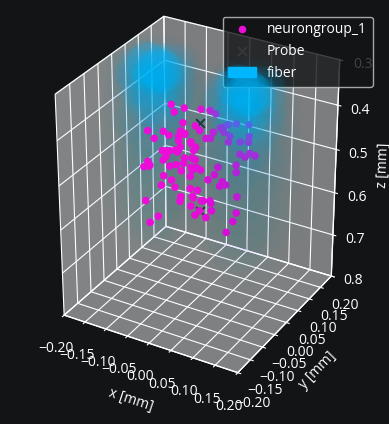
Looks right. Let’s set up the simulation and inject the devices:

sim = cleo.CLSimulator(net)
sim.inject(fibers, ng)
sim.inject(opsin, ng, Iopto_var_name="I")
sim.inject(probe, ng)

CLSimulator(io_processor=None, devices={Probe(name='Probe', save_history=True, signals=[MultiUnitSpiking(name='spikes', brian_objects={<SpikeMonitor, recording from 'spikemonitor_1'>}, probe=..., r_perfect_detection=40. * umetre, r_half_detection=80. * umetre, cutoff_probability=0.01)], probe=NOTHING), Light(name='fiber', save_history=True, value=array([0., 0.]), light_model=OpticFiber(R0=50. * umetre, NAfib=0.37, K=125. * metre ** -1, S=7370. * metre ** -1, ntis=1.36), wavelength=0.473 * umetre, direction=array([0., 0., 1.]), max_value=None, max_value_viz=None), FourStateOpsin(name='ChR2', save_history=True, on_pre='', spectrum=[(400, 0.34), (422, 0.65), (460, 0.96), (470, 1), (473, 1), (500, 0.57), (520, 0.22), (540, 0.06), (560, 0.01), (800, 1.257478763901864e-06), (844, 2.404003519224151e-06), (920, 3.5505282745464387e-06), (940, 3.6984669526525404e-06), (946, 3.6984669526525404e-06), (1000, 2.1081261630119477e-06), (1040, 8.136627295835588e-07), (1080, 2.2190801715915242e-07), (1120, 3.69846695265254e-08)], extrapolate=False, required_vars=[('Iopto', amp), ('v', volt)], g0=114. * nsiemens, gamma=0.00742, phim=2.33e+23 * (second ** -1) / (meter ** 2), k1=4.15 * khertz, k2=0.868 * khertz, p=0.833, Gf0=37.3 * hertz, kf=58.1 * hertz, Gb0=16.1 * hertz, kb=63. * hertz, q=1.94, Gd1=105. * hertz, Gd2=13.8 * hertz, Gr0=0.33 * hertz, E=0. * volt, v0=43. * mvolt, v1=17.1 * mvolt, model="\n        dC1/dt = Gd1*O1 + Gr0*C2 - Ga1*C1 : 1 (clock-driven)\n        dO1/dt = Ga1*C1 + Gb*O2 - (Gd1+Gf)*O1 : 1 (clock-driven)\n        dO2/dt = Ga2*C2 + Gf*O1 - (Gd2+Gb)*O2 : 1 (clock-driven)\n        C2 = 1 - C1 - O1 - O2 : 1\n\n        Theta = int(phi_pre > 0*phi_pre) : 1\n        Hp = Theta * phi_pre**p/(phi_pre**p + phim**p) : 1\n        Ga1 = k1*Hp : hertz\n        Ga2 = k2*Hp : hertz\n        Hq = Theta * phi_pre**q/(phi_pre**q + phim**q) : 1\n        Gf = kf*Hq + Gf0 : hertz\n        Gb = kb*Hq + Gb0 : hertz\n\n        fphi = O1 + gamma*O2 : 1\n        # v1/v0 when v-E == 0 via l'Hopital's rule\n        fv = f_unless_x0(\n            (1 - exp(-(V_VAR_NAME_post-E)/v0)) / ((V_VAR_NAME_post-E)/v1),\n            V_VAR_NAME_post - E,\n            v1/v0\n        ) : 1\n\n        IOPTO_VAR_NAME_post = -g0*fphi*fv*(V_VAR_NAME_post-E)*rho_rel : ampere (summed)\n        rho_rel : 1", extra_namespace={'f_unless_x0': <brian2.core.functions.Function object>})})

Collect training data

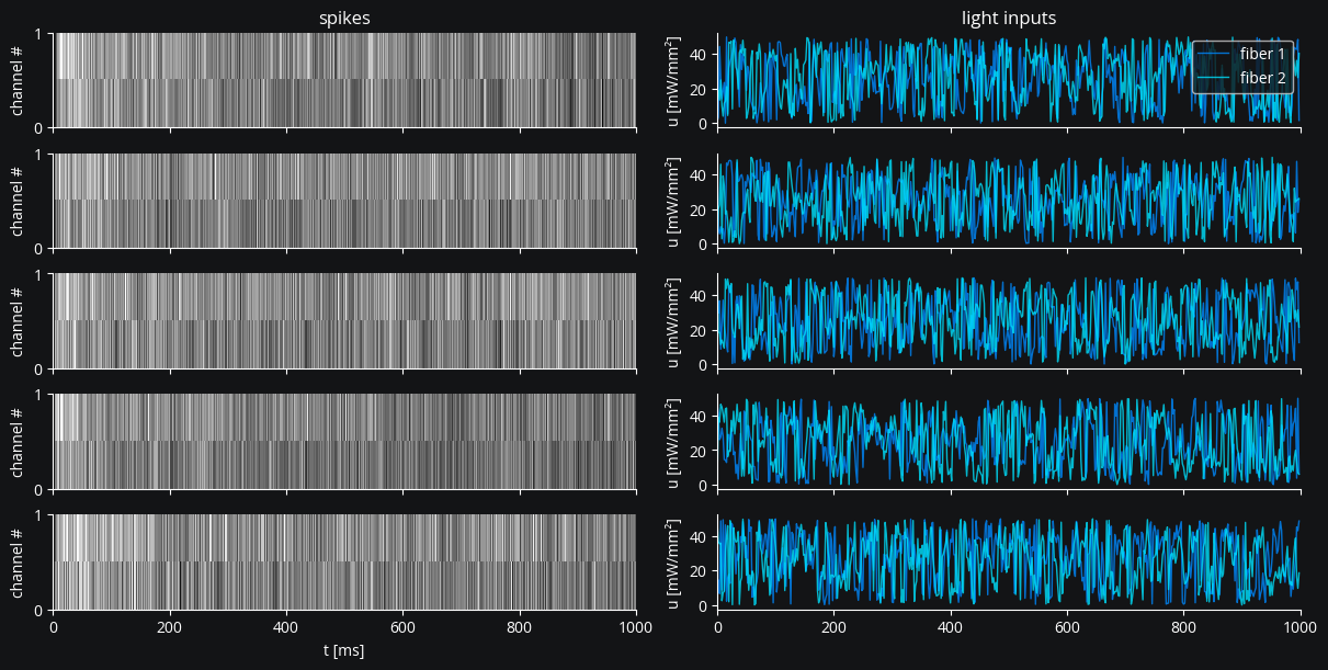
Our goal will be to control two neuron’s firing rates simultaneously. To do this, we will use the LQR technique explained in Bolus et al., 2021 (“State-space optimal feedback control of optogenetically driven neural activity)”. LQR is a model-based technique, and to fit a model of the system’s dynamics, we first need training data. We will generate training data using Gaussian random walk inputs, modulo’ed to a normal stimulation range (0-50 mW/mm²). Here we structure our data into trials, as ldsCtrlEst is designed for. \(u\) represents the input and \(z\) the spike output.

n_trials = 5
n_samp = 500
u = []
z = []
n_u = 2  # 1-dimensional input (just one optogenetic actuator)
n_z = 2  # we'll be controlling two neurons
for trial in range(n_trials):
    u_trial = 10 * np.cumsum(np.random.randn(n_u, n_samp), axis=1) % 50
    u.append(u_trial)
    z.append(np.zeros((n_z, n_samp)))

We configure the LatencyIOProcessor to deliver our pre-computed stimulus and record the results, resetting after each trial:

class TrainingStimIOP(cleo.LatencyIOProcessor):
    i_samp = 0
    i_trial = 0

    # here we just feed in the training inputs and record the outputs
    def process(self, state_dict, t_samp):
        i, t, z_t = state_dict["Probe"]["spikes"]
        z[self.i_trial][:, self.i_samp] = z_t[:n_z]  # just first two neurons
        out = {"fiber": u[self.i_trial][:, self.i_samp] * b2.mwatt / b2.mm2}
        self.i_samp += 1
        return out, t_samp

    # gets called with sim.reset()
    def reset(self):
        self.i_samp = 0


dt = 2 * ms
training_stim_iop = TrainingStimIOP(sample_period=dt)
sim.set_io_processor(training_stim_iop)

for i_trial in range(n_trials):
    training_stim_iop.i_trial = i_trial
    sim.run(n_samp * dt)
    sim.reset()

INFO       No numerical integration method specified for group 'syn_ChR2_neurongroup_1', using method 'euler' (took 0.02s, trying other methods took 0.05s). [brian2.stateupdaters.base.method_choice]

WARNING    'dt' is an internal variable of group 'syn_ChR2_neurongroup_1', but also exists in the run namespace with the value 2. * msecond. The internal variable will be used. [brian2.groups.group.Group.resolve.resolution_conflict]

Let’s plot our training data:

Show code cell source Hide code cell source

fig, axs = plt.subplots(
    n_trials, 2, figsize=(12, 6), layout="compressed", sharex=True, sharey="col"
)

for i, (utrial, ztrial) in enumerate(zip(u, z)):
    # Plot spiking data
    ax_spike = axs[i, 0]
    ax_spike.imshow(
        ztrial,
        aspect="auto",
        cmap="gray",
        extent=[0, (n_samp * dt) / ms, *np.arange(n_z + 1)],
        interpolation="nearest",
        zorder=0,
    )
    ax_spike.set(ylabel="channel #", yticks=range(n_z))
    if i == n_trials - 1:
        ax_spike.set(xlabel="t [ms]")

    # Plot input data
    ax_input = axs[i, 1]
    lines = ax_input.plot(
        np.arange(n_samp) * dt / ms,
        utrial.T,
        alpha=0.8,
        lw=1,
    )
    for i, ln, c in zip(range(n_u), lines, [cu1, cu2]):
        ln.set(color=c, label=f"fiber {i + 1}")
    ax_input.set(ylabel="u [mW/mm²]")
    if i == n_trials - 1:
        ax_input.set(xlabel="t [ms]")

axs[0, 1].legend()
axs[0, 0].set(title="spikes")
axs[0, 1].set(title="light inputs")
plt.show()

Model fitting

Now we have u and z in the form we need for ldsctrlest’s fitting functions: n_trial-length lists of n by n_samp arrays. We will now fit Gaussian linear dynamical systems using the SSID algorithm. See the documentation for more detailed explanations.

import ldsctrlest as lds
import ldsctrlest.gaussian as glds

n_x_fit = 3  # latent dimensionality of system
n_h = 100  # size of block Hankel data matrix
u_train = lds.UniformMatrixList(u, free_dim=2)
z_train = lds.UniformMatrixList(z, free_dim=2)
ssid = glds.FitSSID(n_x_fit, n_h, dt / second, u_train, z_train)
fit, sing_vals = ssid.Run(lds.SSIDWt.kMOESP)
fit_sys_ssid = glds.System(fit)

Here we plot the singular values of the data matrix—we should see a drop at or before our chosen model order if we have a decent fit. We also visualize impulse responses: we should see increases in firing rate for each of the fibers:

n_samp_imp = 50
y_imp = fit_sys_ssid.simulate_imp(n_samp_imp)
t_imp = np.arange(n_samp_imp) * dt / ms

fig, axs = plt.subplots(1, 3, figsize=(2 + n_u * 3, 4), layout="compressed")
axs[0].semilogy(sing_vals[: n_x_fit * 3], linewidth=2)
axs[0].set(ylabel="singular values", xlabel="singular value index")

for i_u in range(n_u):
    ax = axs[i_u + 1]
    lines = ax.plot(t_imp, y_imp[i_u].T, linewidth=2)
    lines[0].set_color(cy1)
    lines[1].set_color(cy2)
    ax.set(title=f"Impulse response for $u_{i_u+1}$", xlabel="time (ms)")


ax.legend(lines, ["$y_1$", "$y_2$"]);

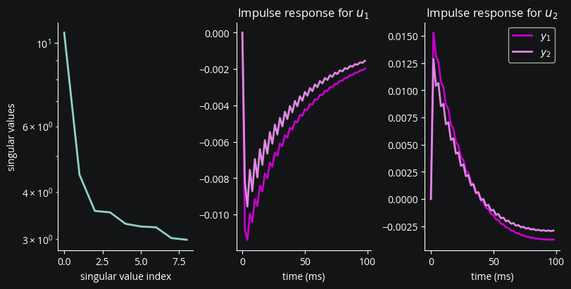
We see a sharp drop in singular values after the first few, which justifies our model order choice. For the impulse responses, we expect both fibers to cause transitory increases in firing rate for both electrodes. Since we see that isn’t the case for the first, let’s try refining our fit with expectation-maximization (EM):

em = glds.FitEM(fit, u_train, z_train)
fit_em = em.Run(
    calc_dynamics=True,
    calc_Q=True,
    calc_init=True,
    calc_output=True,
    calc_measurement=True,
    max_iter=50,
    tol=1e-2,
)
fit_sys_em = glds.System(fit_em)

We’ll plot impulse responses again:

y_imp = fit_sys_em.simulate_imp(n_samp_imp)

fig, axs = plt.subplots(1, 2, figsize=(3 * n_u, 4), layout="compressed")
for i_u in range(n_u):
    ax = axs[i_u]
    lines = ax.plot(t_imp, y_imp[i_u].T, linewidth=2)
    lines[0].set_color(cy1)
    lines[1].set_color(cy2)
    ax.set(title=f"Impulse response for $u_{i_u+1}$", xlabel="time (ms)")

ax.legend(lines, ["$y_1$", "$y_2$"]);

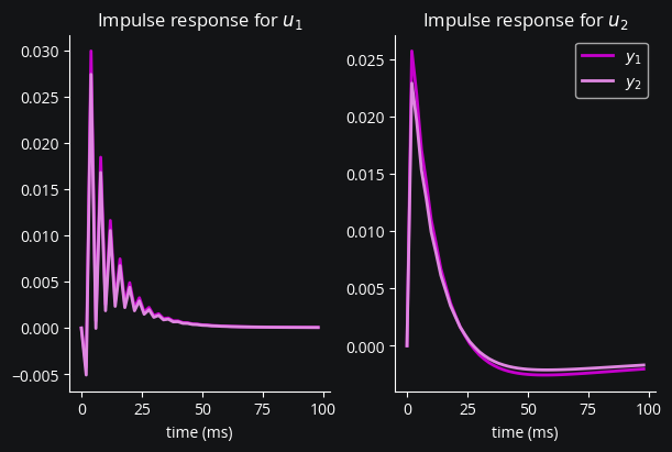
Looking better. Since we can’t visualize singular values, let’s compare the two fits with percent explained variance:

z_arr = np.array(z)


def pct_exp_var(sys, nstep=1):
    x_filt, x_pred, y_pred = sys.nstep_pred_block(u_train, z_train, nstep)
    y_pred = np.array(y_pred)
    assert y_pred.shape == z_arr[:, :, nstep:].shape, y_pred.shape
    corrcoef_mat = np.corrcoef(z_arr[:, :, nstep:].flatten(), y_pred[:, :, :].flatten())
    return corrcoef_mat[0, 1] ** 2


print("SSID r²:", pct_exp_var(fit_sys_ssid))
print("EM r²:", pct_exp_var(fit_sys_em))

SSID r²: 0.04383360173764044
EM r²: 0.13481170536206497

As we suspected from the impulse responses, the EM-refined fit is much better.

LQR optimal controller design

We now use the fit parameters to create the controller system and set additional parameters. The feedback gain, \( K_c \), is especially important, determining how the controller responds to the current “error”—the difference between where the system is (estimated to be) now and where we want it to be. The field of optimal control deals with how to design the controller so as to minimize a cost function reflecting what we care about.

With a linear system (obtained from the fitting procedure above) and quadratic per-timestep cost function \(L\) penalizing distance from the reference \(x^*\) and the input \(u\)

\[ L = \frac{1}{2} (x - x^*)^T Q (x - x^*) + \frac{1}{2} u^T R u \]

we can use the closed-form optimal solution called the Linear Quadratic Regulator (LQR).

\[ K = (R + B^T P B)^{-1}(B^T P A) \quad\quad u = -Kx\]

The \(P\) matrix is obtained by numerically solving the discrete algebraic Riccati equation:

\[ P=A^{T} P A-\left(A^{T} P B\right)\left(R+B^{T} P B\right)^{-1}\left(B^{T} P A\right)+Q \]

# upper and lower bounds on control signal (optic fiber light intensity)
u_lb = 0  # mW/mm2
u_ub = 75  # mW/mm2
controller = glds.Controller(fit_sys_em, u_lb, u_ub)
# careful not to use this anymore since controller made a copy
del fit_sys_em

from scipy.linalg import solve_discrete_are

# cost matrices
# Q reflects how much we care about state error
# we use C'C since we really care about output error, not latent state
Q_cost = controller.sys.C.T @ controller.sys.C
R_cost = 1e-4 * np.eye(n_u)  # reflects how much we care about minimizing the stimulus
A, B = controller.sys.A, controller.sys.B
P = solve_discrete_are(A, B, Q_cost, R_cost)
controller.Kc = np.linalg.inv(R_cost + B.T @ P @ B) @ (B.T @ P @ A)
print(controller)
print("For controlled system dynamics A - BK:")
print("eigvals:", np.linalg.eigvals(A - B @ controller.Kc))
print("magnitude of eigvals:", np.abs(np.linalg.eigvals(A - B @ controller.Kc)))

 ********** SYSTEM ********** 
x: 
  -27.0134
  -14.3165
   -2.7832

P: 
   11.5611    4.4943    0.0430
    4.4943    2.4885    0.3463
    0.0430    0.3463   11.7346

A: 
   0.9613   0.0973   0.0392
   0.0294   0.8609   0.0877
  -0.0127   0.0470  -0.7268

B: 
   0.0153   0.0056
  -0.0133  -0.0344
  -0.0591  -0.0027

g: 
   1.0000
   1.0000

m: 
        0
        0
        0

Q: 
   0.3636   0.1986   1.4124
   0.1986   0.2662   1.3413
   1.4124   1.3413   8.5356

Q_m: 
   1.0000e-06            0            0
            0   1.0000e-06            0
            0            0   1.0000e-06

d: 
   15.0531
   13.3232

C: 
   0.3976  -0.7091   0.3339
   0.3415  -0.6354   0.3171

y: 
   13.5351
   12.3129

R: 
   10.7560    1.1165
    1.1165   10.7561

g_design :    1.0000
   1.0000

u_lb : 0
u_ub : 75

For controlled system dynamics A - BK:
eigvals: [ 0.98651763  0.06694736 -0.2470999 ]
magnitude of eigvals: [0.98651763 0.06694736 0.2470999 ]

We now configure a LatencyIOProcessor to use our controller:

y_ref = np.mean(z) * 0.75  # target rate per timebin


class CtrlLoop(cleo.LatencyIOProcessor):
    def __init__(self, sample_period, controller):
        super().__init__(sample_period)
        self.controller = controller
        self.sys = controller.sys
        self.do_control = False  # allows us to turn on and off control

        # for post hoc visualization/analysis:
        self.x_hat = np.empty((n_x_fit, 0))
        self.y_hat = np.empty((n_z, 0))
        self.z = np.empty((n_z, 0))

    def process(self, state_dict, t_samp):
        i, t, z_t = state_dict["Probe"]["spikes"]
        z_t = z_t[:n_z].reshape((-1, 1))  # just first n_z neurons
        self.controller.y_ref = np.ones((n_z, 1)) * y_ref

        u_t = self.controller.ControlOutputReference(z_t, do_control=self.do_control)
        out = {fibers.name: u_t.squeeze() * b2.mwatt / b2.mm2}

        # record variables from this timestep
        self.y_hat = np.hstack([self.y_hat, self.sys.y])
        self.x_hat = np.hstack([self.x_hat, self.sys.x])
        self.z = np.hstack((self.z, z_t))

        return out, t_samp + 3 * ms  # 3 ms delay


ctrl_loop = CtrlLoop(sample_period=dt, controller=controller)

Run the experiment

We’ll now run the simulation with and without control to compare.

sim.set_io_processor(ctrl_loop)
sim.reset()  # only needed when rerunning
T0 = 200 * ms
sim.run(T0)

ctrl_loop.do_control = True
T1 = 1000 * ms
sim.run(T1)

Now we plot the results to see how well the controller was able to match the desired firing rate:

fig, (ax1, ax2) = plt.subplots(2, 1, sharex=True)
ax1.set(ylabel="spikes/s", title="real-time estimated firing rates")
ax1.plot(
    ctrl_loop.t_samp / ms,
    ctrl_loop.y_hat[0] / dt,
    c=cy1,
    alpha=0.7,
    label="$\\hat{y}_1$",
)
ax1.plot(
    ctrl_loop.t_samp / ms,
    ctrl_loop.y_hat[1] / dt,
    c=cy2,
    alpha=0.7,
    label="$\\hat{y}_2$",
)
ax1.hlines((y_ref / dt) / Hz, T0 / ms, (T0 + T1) / ms, color="green", label="reference")
ax1.hlines(0, 0, T0 / ms, color="green")
ax1.axvline(T0 / ms, c="xkcd:red", linestyle=":", label="ctrl on")
ax1.legend(loc="right")
ax2.plot(fibers.t / b2.ms, fibers.irradiance_[:, 0], c=cu1)
ax2.plot(fibers.t / b2.ms, fibers.irradiance_[:, 1], c=cu2)
ax2.set(xlabel="t (ms)", ylabel="u (mW/mm$^2$)", title="input signal");

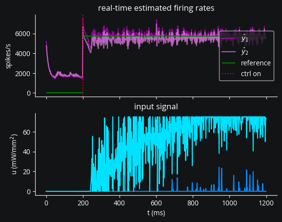
Looks all right, but in addition to the system’s estimated firing rate let’s count the spikes over the control period to see how well we hit the target on average. We also plot a Gaussian-smoothed post hoc estimated firing rate:

from scipy.ndimage import gaussian_filter1d

i_baseline = ctrl_loop.t_samp < T0
i_static = (ctrl_loop.t_samp >= T0) & (ctrl_loop.t_samp < T0 + T1)
print("Results (spikes/second):")
print("baseline =", np.sum(ctrl_loop.z[:, i_baseline], axis=1) / T0)
print("target =", y_ref / dt)
print(
    "lqr achieved =",
    (np.sum(ctrl_loop.z[:, i_static], axis=1) / T1).round(1),
)

win_len = 25 * ms / dt
smoothed = gaussian_filter1d(ctrl_loop.z, sigma=win_len, axis=1) / dt
plt.axhline(y_ref / dt / b2.Hz, c="g")
plt.axvline(T0 / ms, c="r", ls=":")
plt.xlabel("t (ms)")
plt.ylabel("spikes/s")
plt.title("Gaussian-smoothed firing rate")
plt.plot(ctrl_loop.t_samp / ms, smoothed[0], c=cy1)
plt.plot(ctrl_loop.t_samp / ms, smoothed[1], c=cy2);

Results (spikes/second):
baseline = [0.425 0.35 ] kHz
target = 5.742825 kHz
lqr achieved = [5.606 5.053] kHz

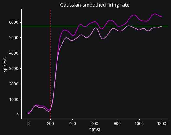
Looks like the system-estimated firing rate was close to the truth.

Conclusion

As a recap, in this tutorial we’ve seen how to:

• inject optogenetic stimulation into an existing Brian network

• inject an electrode into an existing Brian network to record spikes

• generate training data and fit a Gaussian linear dynamical system to the spiking output using ldsctrlest

• configure an ldsctrlest LQR controller based on that linear system and design optimal gains

• use that controller in running a complete simulated feedback control experiment