On-off control#
Here we will see how to set up a minimum, working closed loop with a very simple threshold-triggered control scheme.
Preamble:
from brian2 import *
from cleosim import *

import matplotlib.pyplot as plt

utilities.style_plots_for_docs()

# the default cython compilation target isn't worth it for
# this trivial example
prefs.codegen.target = "numpy"
INFO       Cache size for target 'cython': 1933664869 MB.
You can call clear_cache('cython') to delete all files from the cache or manually delete files in the '/home/kyle/.cython/brian_extensions' directory. [brian2]
Set up network#
We will use a simple leaky integrate-and-fire network with Poisson spike train input. We use Brian’s standard SpikeMonitor to view resulting spikes here for simplicity, but see the electrodes tutorial for a more realistic electrode recording scheme.
n = 10
population = NeuronGroup(n, '''
            dv/dt = (-v - 70*mV + Rm*I) / tau : volt
            tau: second
            Rm: ohm
            I: amp''',
        threshold='v>-50*mV',
        reset='v=-70*mV'
)
population.tau = 10*ms
population.Rm = 100*Mohm
population.I = 0*mA
population.v = -70*mV

input_group = PoissonGroup(n, np.linspace(0, 100, n)*Hz + 10*Hz)

S = Synapses(input_group, population, on_pre='v+=5*mV')
S.connect(condition='abs(i-j)<=3')

pop_mon = SpikeMonitor(population)

net = Network([population, input_group,S, pop_mon])

print("Recorded population's equations:")
population.user_equations
Recorded population's equations:
Run simulation#
net.run(200*ms)
INFO No numerical integration method specified for group 'neurongroup', using method 'exact' (took 0.08s). [brian2.stateupdaters.base.method_choice]
sptrains = pop_mon.spike_trains()
fig, ax = plt.subplots()
ax.eventplot([t / ms for t in sptrains.values()], lineoffsets=list(sptrains.keys()))
ax.set(title='population spiking', ylabel='neuron index', xlabel='time (ms)')
[Text(0.5, 1.0, 'population spiking'),
 Text(0, 0.5, 'neuron index'),
 Text(0.5, 0, 'time (ms)')]

Because lower neuron indices receive very little input, we see no spikes for neuron 0. Let’s change that with closed-loop control.
IO processor setup#
We use the IOProcessor class to define interactions with the network.
To achieve our goal of making neuron 0 fire, we’ll use a contrived, simplistic setup where
the recorder reports the voltage of a given neuron (of index 5 in our case),
the controller outputs a pulse whenever that voltage is below a certain threshold, and
the stimulator applies that pulse to the specified neuron.
So if everything is wired correctly, we’ll see bursts of activity in just the first neuron.
from cleosim.recorders import RateRecorder, VoltageRecorder
from cleosim.stimulators import StateVariableSetter

i_rec = int(n / 2)
i_ctrl = 0
sim = CLSimulator(net)
v_rec = VoltageRecorder("rec")
sim.inject_recorder(v_rec, population[i_rec])
sim.inject_stimulator(
    StateVariableSetter("stim", variable_to_ctrl="I", unit=nA), population[i_ctrl]
)
We need to implement the LatencyIOProcessor object. For a more sophisticated case we’d use ProcessingBlock objects to decompose
the computation in the process function.
from cleosim.processing import LatencyIOProcessor

trigger_threshold = -60*mV
class ReactivePulseIOProcessor(LatencyIOProcessor):
    def __init__(self, pulse_current=1):
        super().__init__(sample_period_ms=1)
        self.pulse_current = pulse_current
        self.out = {}

    def process(self, state_dict, time_ms):
        v = state_dict['rec']
        if v is not None and v < trigger_threshold:
            self.out['stim'] = self.pulse_current
        else:
            self.out['stim'] = 0

        return (self.out, time_ms)

sim.set_io_processor(ReactivePulseIOProcessor(pulse_current=1))
And run the simulation:
sim.run(200*ms)
fig, (ax1, ax2) = plt.subplots(2, 1, sharex=True)
ax1.plot(pop_mon.t / ms, pop_mon.i[:], "|")
ax1.plot(
    pop_mon.t[pop_mon.i == i_ctrl] / ms,
    pop_mon.i[pop_mon.i == i_ctrl],
    "|",
    c="#C500CC",
)
ax1.set(title="population spiking", ylabel="neuron index", xlabel="time (ms)")
ax2.fill_between(
    v_rec.mon.t / ms, (v_rec.mon.v.T < trigger_threshold)[:, 0], color="#C500CC"
)
ax2.set(title="pulses", xlabel="time (ms)", ylabel="pulse on/off (1/0)", yticks=[0, 1])
plt.tight_layout()
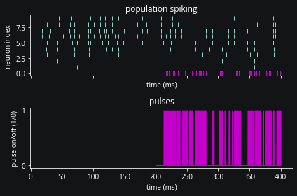
Yes, we see the IO processor triggering pulses as expected. And here’s a plot of neuron 5’s voltage to confirm that those pulses are indeed where we expect them to be, whenever the voltage is below -60 mV.
fig, ax = plt.subplots()
ax.set(title=f"Voltage for neuron {i_rec}", ylabel="v (mV)", xlabel='time (ms)')
ax.plot(v_rec.mon.t/ms, v_rec.mon.v.T / mV);
ax.hlines(-60, 0, 400, color='#c500cc');
ax.legend(['v', 'threshold'], loc='upper right');

Conclusion#
In this tutorial we’ve seen the basics of configuring an IOProcessor to implement a closed-loop intervention on a Brian network simulation.