Electrode recording#
How to insert electrodes to measure different spiking and extracellular signals from a Brian network simulation.
Preamble:
from brian2 import *  # includes numpy
import cleo
from cleo import *
# the default cython compilation target isn't worth it for
# this trivial example
prefs.codegen.target = "numpy"
np.random.seed(1919)

cleo.utilities.style_plots_for_docs()

# colors
c = {
    'light': '#df87e1',
    'main': '#C500CC',
    'dark': '#8000B4',
    'exc': '#d6755e',
    'inh': '#056eee',
    'accent': '#36827F',
}
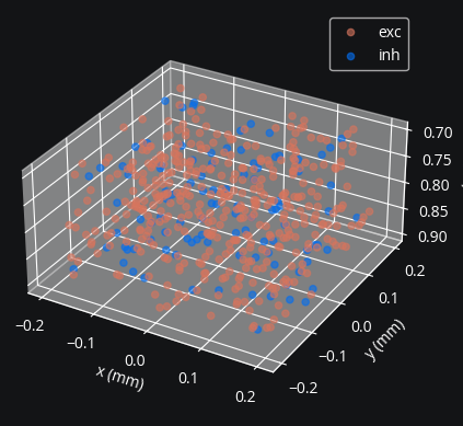
Network setup#
First we create a toy E-I network with Poisson firing rates and assign coordinates:
N = 500
n_e = int(N * 0.8)
n_i = int(N * 0.2)

exc = PoissonGroup(n_e, 10 * Hz, name="exc")
inh = PoissonGroup(n_i, 30 * Hz, name="inh")

net = Network([exc, inh])
sim = CLSimulator(net)

cleo.coords.assign_coords_rand_rect_prism(
    exc, xlim=(-0.2, 0.2), ylim=(-0.2, 0.2), zlim=(0.7, 0.9)
)
cleo.coords.assign_coords_rand_rect_prism(
    inh, xlim=(-0.2, 0.2), ylim=(-0.2, 0.2), zlim=(0.7, 0.9)
)
cleo.viz.plot(exc, inh, colors=[c['exc'], c['inh']], scatterargs={'alpha': .6})
(<Figure size 640x480 with 1 Axes>,
 <Axes3D: xlabel='x (mm)', ylabel='y (mm)', zlabel='z (mm)'>)
Specifying electrode coordinates#
Now we insert an electrode shank probe in the center of the population by injecting an Probe device.
Note that Probe takes arbitrary coordinates as arguments, so you can place contacts wherever you wish. However, the cleo.ephys module provides convenience functions to easily generate coordinates common in NeuroNexus probes. Here are some examples:
from cleo import ephys
from mpl_toolkits.mplot3d import Axes3D

array_length = 0.4 * mm  # length of the array itself, not the shank
tetr_coords = ephys.tetrode_shank_coords(array_length, tetrode_count=3)
poly2_coords = ephys.poly2_shank_coords(
    array_length, channel_count=32, intercol_space=50 * umeter
)
poly3_coords = ephys.poly3_shank_coords(
    array_length, channel_count=32, intercol_space=30 * umeter
)
# by default start_location (location of first contact) is at (0, 0, 0)
single_shank = ephys.linear_shank_coords(
    array_length, channel_count=8, start_location=(-0.2, 0, 0) * mm
)
# tile vector determines length and direction of tiling (repeating)
multishank = ephys.tile_coords(single_shank, num_tiles=3, tile_vector=(0.4, 0, 0) * mm)

fig = plt.figure(figsize=(8, 8))
fig.suptitle("Example array configurations")
for i, (coords, title) in enumerate(
    [
        (tetr_coords, "3-tetrode shank"),
        (poly2_coords, "32-channel Poly2 shank"),
        (poly3_coords, "32-channel Poly3 shank"),
        (multishank, "Multi-shank"),
    ],
    start=1,
):
    ax = fig.add_subplot(2, 2, i, projection="3d")
    x, y, z = coords.T / umeter
    ax.scatter(x, y, z, marker="x", c="black")
    ax.set(
        title=title,
        xlabel="x (μm)",
        ylabel="y (μm)",
        zlabel="z (μm)",
        xlim=(-200, 200),
        ylim=(-200, 200),
        zlim=(400, 0),
    )

As seen above, the tile_coords function can be used to repeat a single shank to produce coordinates for a multi-shank probe. Likewise it can be used to repeat multi-shank coordinates to achieve a 3D recording array (what NeuroNexus calls a MatrixArray).
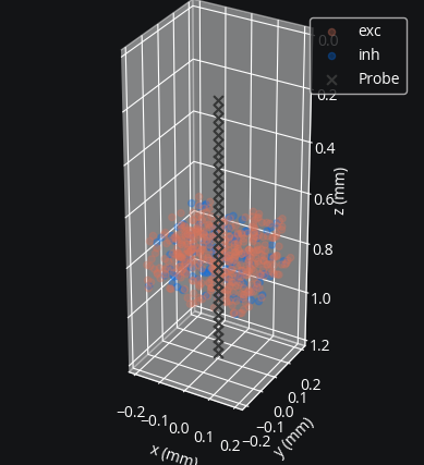
For our example we will use a simple linear array. We configure the probe so it has 32 contacts ranging from 0.2 to 1.2 mm in depth. We could specify the orientation, but by default shank coordinates extend downwards (in the positive z direction).
We can add the electrode to the plotting function to visualize it along with the neurons:
coords = ephys.linear_shank_coords(1 * mm, 32, start_location=(0, 0, 0.2) * mm)
probe = ephys.Probe(coords)
cleo.viz.plot(
    exc, inh, colors=[c['exc'], c['inh']], zlim=(0, 1.2), devices=[probe], scatterargs={'alpha': .3}
)
(<Figure size 640x480 with 1 Axes>,
 <Axes3D: xlabel='x (mm)', ylabel='y (mm)', zlabel='z (mm)'>)
Specifying signals to record#
This looks right, but we need to specify what signals we want to pick up with our electrode. Let’s try the two basic spiking signals and an LFP approximation for point neurons.
The two spiking signals (sorted and multi-unit) take the same parameters, mainly r_perfect_detection, within which all spikes will be detected, and r_half_detection, at which distance a spike has only a 50% chance of being detected. My choice to set these parameters at 50 and 100 μm is arbitary, though from at least some published data that seems reasonable.
We use default parameters for the Teleńczuk kernel LFP approximation method (TKLFP), but will need to specify cell type (excitatory or inhibitory) and sampling period (if unavailable from a connected IO processor) upon injection.
mua = ephys.MultiUnitSpiking(
    r_perfect_detection=0.05 * mm,
    r_half_detection=0.1 * mm,
    save_history=True,
)
ss = ephys.SortedSpiking(0.05 * mm, 0.1 * mm, save_history=True)
tklfp = ephys.TKLFPSignal(save_history=True)

probe.add_signals(mua, ss, tklfp)

from cleo.ioproc import RecordOnlyProcessor
sim.set_io_processor(RecordOnlyProcessor(sample_period_ms=1))
sim.inject(probe, exc, tklfp_type="exc")
sim.inject(probe, inh, tklfp_type="inh")
CLSimulator(io_processor=<cleo.ioproc.base.RecordOnlyProcessor object at 0x7f87cac0f790>, devices={Probe(brian_objects={<SpikeMonitor, recording from 'spikemonitor_5'>, <SpikeMonitor, recording from 'spikemonitor_1'>, <SpikeMonitor, recording from 'spikemonitor'>, <SpikeMonitor, recording from 'spikemonitor_4'>, <SpikeMonitor, recording from 'spikemonitor_2'>, <SpikeMonitor, recording from 'spikemonitor_3'>}, sim=..., name='Probe', signals=[MultiUnitSpiking(name='MultiUnitSpiking', brian_objects={<SpikeMonitor, recording from 'spikemonitor_3'>, <SpikeMonitor, recording from 'spikemonitor'>}, probe=..., r_perfect_detection=50. * umetre, r_half_detection=100. * umetre, cutoff_probability=0.01, save_history=True), SortedSpiking(name='SortedSpiking', brian_objects={<SpikeMonitor, recording from 'spikemonitor_1'>, <SpikeMonitor, recording from 'spikemonitor_4'>}, probe=..., r_perfect_detection=50. * umetre, r_half_detection=100. * umetre, cutoff_probability=0.01, save_history=True), TKLFPSignal(name='TKLFPSignal', brian_objects={<SpikeMonitor, recording from 'spikemonitor_2'>, <SpikeMonitor, recording from 'spikemonitor_5'>}, probe=..., uLFP_threshold_uV=0.001, save_history=True)], probe=NOTHING)})
Simulation and results#
Now we’ll run the simulation:
sim.run(150*ms)
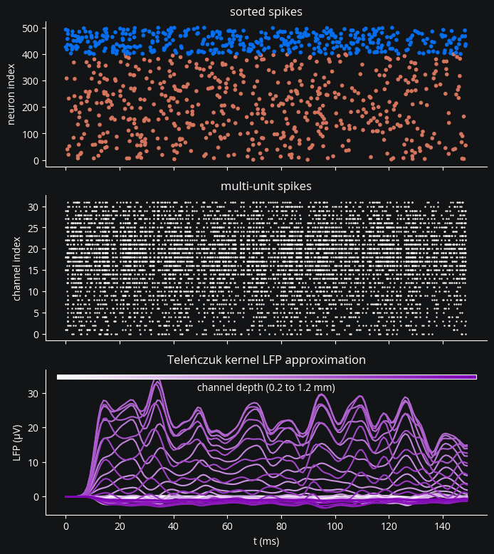
And plot the output of the three signals we’ve recorded:
from matplotlib.colors import ListedColormap, LinearSegmentedColormap
fig, axs = plt.subplots(3, 1, figsize=(8, 9), sharex=True)

# assuming all neurons are detectable for c=ss.i >= n_e to work
# in practice this will often not be the case and we'd have to map
# from probe index to neuron group index using ss.i_probe_by_i_ng.inverse
exc_inh_cmap = ListedColormap([c['exc'], c['inh']])
axs[0].scatter(ss.t_ms, ss.i, marker=".", c=ss.i >= n_e, cmap=exc_inh_cmap)
axs[0].set(title="sorted spikes", ylabel="neuron index")

axs[1].scatter(mua.t_ms, mua.i, marker=".", s=2, c='white')
axs[1].set(title="multi-unit spikes", ylabel="channel index")

lines = axs[2].plot(tklfp.lfp_uV)
axs[2].set(
    title="Teleńczuk kernel LFP approximation", xlabel="t (ms)", ylabel="LFP (μV)"
)

# color-code channel depth
from mpl_toolkits.axes_grid1.inset_locator import inset_axes
depth_cmap = LinearSegmentedColormap.from_list('cleo', ['white', c['dark']])
axins = inset_axes(axs[2], width='95%', height='3%', loc="upper center")
for i in range(32):
    l = lines[i]
    l.set_color(depth_cmap(i / 31))
from matplotlib.colors import Normalize
channel_mappable = plt.cm.ScalarMappable(Normalize(0, 1.2), depth_cmap)
fig.colorbar(
    channel_mappable,
    cax=axins,
    orientation="horizontal",
    ticks=[],
    label="channel depth (0.2 to 1.2 mm)",
);
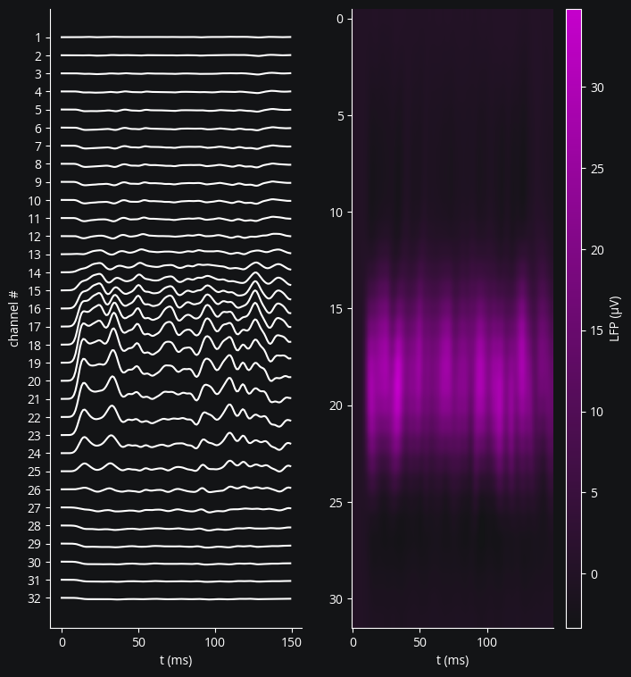
Or, to see the LFP as a function of depth better:
fig, axs = plt.subplots(1, 2, figsize=(8, 9))
channel_offsets = -12 * np.arange(32)
lfp_to_plot = tklfp.lfp_uV + channel_offsets
axs[0].plot(lfp_to_plot, color="w")
axs[0].set(
    yticks=channel_offsets,
    yticklabels=range(1, 33),
    xlabel="t (ms)",
    ylabel="channel #",
)
cmap = LinearSegmentedColormap.from_list('lfp', ['#131416', c['main']])
im = axs[1].imshow(tklfp.lfp_uV.T, aspect="auto", cmap=cmap)
axs[1].set(xlabel="t (ms)")
fig.colorbar(im, aspect=40, label="LFP (μV)")
<matplotlib.colorbar.Colorbar at 0x7f87ca70dc60>