Overview

Introduction

Who is this package for?

Cleo (Closed-Loop, Electrophysiology, and Optophysiology experiment simulation testbed) is a Python package developed to bridge theory and experiment for mesoscale neuroscience. We envision two primary uses cases:

1. For prototyping closed-loop control of neural activity in silico. Animal experiments are costly to set up and debug, especially with the added complexity of real-time intervention—our aim is to enable researchers, given a decent spiking model of the system of interest, to assess whether the type of control they desire is feasible and/or what configuration(s) would be most conducive to their goals.

2. The complexity of experimental interfaces means it’s not always clear what a model would look like in a real experiment. Cleo can help anyone interested in observing or manipulating a model while taking into account the constraints present in real experiments. Because Cleo is built around the Brian simulator, we especially hope this is helpful for existing Brian users who for whatever reason would like a convenient way to inject recorders (e.g., electrodes or 2P imaging) or stimulators (e.g., optogenetics) into the core network simulation.

What is closed-loop control?

In short, determining the inputs to deliver to a system from its outputs. In neuroscience terms, making the stimulation parameters a function of the data recorded in real time.

Structure and design

Cleo wraps a spiking network simulator and allows for the injection of stimulators and/or recorders. The models used to emulate these devices are often non-trivial to implement or use in a flexible manner, so Cleo aims to make device injection and configuration as painless as possible, requiring minimal modification to the original network.

Cleo also orchestrates communication between the simulator and a user-configured IOProcessor object, modeling how experiment hardware takes samples, processes signals, and controls stimulation devices in real time.

For an explanation of why we choose to prioritize spiking network models and how we chose Brian as the underlying simulator, see Design rationale.

Why closed-loop control in neuroscience?

Fast, real-time, closed-loop control of neural activity enables intervention in processes that are too fast or unpredictable to control manually or with pre-defined stimulation, such as sensory information processing, motor planning, and oscillatory activity. Closed-loop control in a reactive sense enables the experimenter to respond to discrete events of interest, such as the arrival of a traveling wave or sharp wave ripple, whereas feedback control deals with driving the system towards a desired point or along a desired state trajectory. The latter has the effect of rejecting noise and disturbances, reducing variability across time and across trials, allowing the researcher to perform inference with less data and on a finer scale. Additionally, closed-loop control can compensate for model mismatch, allowing it to reach more complex targets where open-loop control based on imperfect models is bound to fail.

Installation

Make sure you have Python ≥ 3.7, then use pip: pip install cleosim.

Caution

The name on PyPI is cleosim since cleo was already taken, but in code it is still used as import cleo. The other Cleo appears to actually be a fairly well developed package, so I’m sorry if you need to use it along with this Cleo in the same environment. In that case, there are workarounds.

Or, if you’re a developer, install poetry and run poetry install from the repository root.

Usage

Brian network model

The starting point for using Cleo is a Brian spiking neural network model of the system of interest. For those new to Brian, the docs are a great resource. If you have a model built with another simulator or modeling language, you may be able to import it to Brian via NeuroML.

Perhaps the biggest change you may have to make to an existing model to make it compatible with Cleo’s optogenetics and electrode recording is to give the neurons of interest coordinates in space. See the tutorials or the cleo.coords module for more info.

You’ll need your model in a Brian Network object before you move on. E.g.,:

import brian2 as b2
ng = b2.NeuronGroup( # a simple population of 100 LIF neurons
    500,
    """dv/dt = (-v - 70*mV + (500*Mohm)*Iopto + 2*xi*sqrt(tau_m)*mvolt) / tau_m : volt
    Iopto : amp""",
    threshold='v>-50*mV',
    reset='v=-70*mV',
    namespace={'tau_m': 20*b2.ms},
)
ng.v = -70*b2.mV
net = b2.Network(ng)

Your neurons need x, y, and z coordinates for Cleo’s spatially defined recording and stimulation models to work:

import cleo
cleo.coords.assign_coords_rand_rect_prism(
    ng, xlim=(-0.2, 0.2), ylim=(-0.2, 0.2), zlim=(0.2, 1), unit=b2.mm
)

CLSimulator

Once you have a network model, you can construct a CLSimulator object:

sim = cleo.CLSimulator(net)

The simulator object wraps the Brian network and coordinates device injection, processing input and output, and running the simulation.

Recording

Recording devices take measurements of the Brian network. To use a Recorder, you must inject it into the simulator via cleo.CLSimulator.inject(). The recorder will only record from the neuron groups specified on injection, allowing for such scenarios as singling out a cell type to record from. Some extremely simple implementations (which do little more than wrap Brian monitors) are available in the cleo.recorders module. See the Electrode recording and All-optical control tutorials for more detail on how to record from a simulation more realistically, but here’s a quick example of how to record multi-unit spiking activity with an electrode:

# configure and inject a 32-channel shank
coords = cleo.ephys.linear_shank_coords(
    array_length=1*b2.mm, channel_count=32, start_location=(0, 0, 0.2)*b2.mm
)
mua = cleo.ephys.MultiUnitSpiking(
    r_perfect_detection=20 * b2.um,
    r_half_detection=40 * b2.um,
)
probe = cleo.ephys.Probe(coords, signals=[mua])
sim.inject(probe, ng)

CLSimulator(io_processor=None, devices={Probe(name='Probe', save_history=True, signals=[MultiUnitSpiking(name='MultiUnitSpiking', brian_objects={<SpikeMonitor, recording from 'spikemonitor'>}, probe=..., r_perfect_detection=20. * umetre, r_half_detection=40. * umetre, cutoff_probability=0.01)], probe=NOTHING)})

Stimulation

Stimulator devices manipulate the Brian network, and are likewise inject()ed into the simulator, into specified neuron groups. Optogenetics (1P and 2P) is the main stimulation modality currently implemented by Cleo. This requires injection of both a light source and an opsin—see the Optogenetic stimulation and All-optical control tutorials for more detail.

fiber = cleo.light.Light(
    coords=(0, 0, 0.5)*b2.mm,
    light_model=cleo.light.fiber473nm(),
    wavelength=473*b2.nmeter
)
chr2 = cleo.opto.chr2_4s()
sim.inject(fiber, ng).inject(chr2, ng)

CLSimulator(io_processor=None, devices={Light(name='Light', save_history=True, value=array([0.]), light_model=OpticFiber(R0=100. * umetre, NAfib=0.37, K=125. * metre ** -1, S=7370. * metre ** -1, ntis=1.36), wavelength=0.473 * umetre, direction=array([0., 0., 1.]), max_Irr0_mW_per_mm2=None, max_Irr0_mW_per_mm2_viz=None), FourStateOpsin(name='ChR2', save_history=True, on_pre='', spectrum=[(400, 0.34), (422, 0.65), (460, 0.96), (470, 1), (473, 1), (500, 0.57), (520, 0.22), (540, 0.06), (560, 0.01)], required_vars=[('Iopto', amp), ('v', volt)], g0=114. * nsiemens, gamma=0.00742, phim=2.33e+23 * (second ** -1) / (meter ** 2), k1=4.15 * khertz, k2=0.868 * khertz, p=0.833, Gf0=37.3 * hertz, kf=58.1 * hertz, Gb0=16.1 * hertz, kb=63. * hertz, q=1.94, Gd1=105. * hertz, Gd2=13.8 * hertz, Gr0=0.33 * hertz, E=0. * volt, v0=43. * mvolt, v1=17.1 * mvolt, model="\n        dC1/dt = Gd1*O1 + Gr0*C2 - Ga1*C1 : 1 (clock-driven)\n        dO1/dt = Ga1*C1 + Gb*O2 - (Gd1+Gf)*O1 : 1 (clock-driven)\n        dO2/dt = Ga2*C2 + Gf*O1 - (Gd2+Gb)*O2 : 1 (clock-driven)\n        C2 = 1 - C1 - O1 - O2 : 1\n\n        Theta = int(phi_pre > 0*phi_pre) : 1\n        Hp = Theta * phi_pre**p/(phi_pre**p + phim**p) : 1\n        Ga1 = k1*Hp : hertz\n        Ga2 = k2*Hp : hertz\n        Hq = Theta * phi_pre**q/(phi_pre**q + phim**q) : 1\n        Gf = kf*Hq + Gf0 : hertz\n        Gb = kb*Hq + Gb0 : hertz\n\n        fphi = O1 + gamma*O2 : 1\n        # v1/v0 when v-E == 0 via l'Hopital's rule\n        fv = f_unless_x0(\n            (1 - exp(-(V_VAR_NAME_post-E)/v0)) / ((V_VAR_NAME_post-E)/v1),\n            V_VAR_NAME_post - E,\n            v1/v0\n        ) : 1\n\n        IOPTO_VAR_NAME_post = -g0*fphi*fv*(V_VAR_NAME_post-E)*rho_rel : ampere (summed)\n        rho_rel : 1", extra_namespace={'f_unless_x0': <brian2.core.functions.Function object at 0x7f2ee4539880>}), Probe(name='Probe', save_history=True, signals=[MultiUnitSpiking(name='MultiUnitSpiking', brian_objects={<SpikeMonitor, recording from 'spikemonitor'>}, probe=..., r_perfect_detection=20. * umetre, r_half_detection=40. * umetre, cutoff_probability=0.01)], probe=NOTHING)})

Note

Markov opsin kinetics models require target neurons to have membrane potentials in realistic ranges and an Iopto term defined in amperes. If you need to interface with a model without these features, you may want to use the simplified ProportionalCurrentOpsin. You can find more details, including a comparison between the two model types, in the optogenetics tutorial.

Note

Recorders and stimulators need unique names which serve as keys to access/set values in the IOProcessor’s input/output dictionaries. The name defaults to the class name, but you can specify it on construction.

I/O Processor

Just as in a real experiment where the experiment hardware must be connected to signal processing equipment and/or computers for recording and control, the CLSimulator must be connected to an IOProcessor. If you are only recording, you may want to use the RecordOnlyProcessor. Otherwise you will want to implement the LatencyIOProcessor, which not only takes samples at the specified rate, but processes the data and delivers input to the network after a user-defined delay, emulating the latency inherent in real experiments. This is done by creating a subclass and defining the process() function:

class MyProcessor(cleo.ioproc.LatencyIOProcessor):
    def process(self, state_dict, sample_time_ms):
        # state_dict contains a {'recorder_name': value} dict of network.
        i_spikes, t_ms_spikes, y_spikes = state_dict['Probe']['MultiUnitSpiking']
        # on-off control
        irr0_mW_per_mm2 = 5 if len(i_spikes) < 10 else 0
        # output is a {'stimulator_name': value} dict and output time
        return {'Light': irr0_mW_per_mm2}, sample_time_ms + 3  # (3 ms delay)

sim.set_io_processor(MyProcessor(sample_period_ms=1))

CLSimulator(io_processor=MyProcessor(sample_period_ms=1, sampling='fixed', processing='parallel'), devices={Light(name='Light', save_history=True, value=array([0.]), light_model=OpticFiber(R0=100. * umetre, NAfib=0.37, K=125. * metre ** -1, S=7370. * metre ** -1, ntis=1.36), wavelength=0.473 * umetre, direction=array([0., 0., 1.]), max_Irr0_mW_per_mm2=None, max_Irr0_mW_per_mm2_viz=None), FourStateOpsin(name='ChR2', save_history=True, on_pre='', spectrum=[(400, 0.34), (422, 0.65), (460, 0.96), (470, 1), (473, 1), (500, 0.57), (520, 0.22), (540, 0.06), (560, 0.01)], required_vars=[('Iopto', amp), ('v', volt)], g0=114. * nsiemens, gamma=0.00742, phim=2.33e+23 * (second ** -1) / (meter ** 2), k1=4.15 * khertz, k2=0.868 * khertz, p=0.833, Gf0=37.3 * hertz, kf=58.1 * hertz, Gb0=16.1 * hertz, kb=63. * hertz, q=1.94, Gd1=105. * hertz, Gd2=13.8 * hertz, Gr0=0.33 * hertz, E=0. * volt, v0=43. * mvolt, v1=17.1 * mvolt, model="\n        dC1/dt = Gd1*O1 + Gr0*C2 - Ga1*C1 : 1 (clock-driven)\n        dO1/dt = Ga1*C1 + Gb*O2 - (Gd1+Gf)*O1 : 1 (clock-driven)\n        dO2/dt = Ga2*C2 + Gf*O1 - (Gd2+Gb)*O2 : 1 (clock-driven)\n        C2 = 1 - C1 - O1 - O2 : 1\n\n        Theta = int(phi_pre > 0*phi_pre) : 1\n        Hp = Theta * phi_pre**p/(phi_pre**p + phim**p) : 1\n        Ga1 = k1*Hp : hertz\n        Ga2 = k2*Hp : hertz\n        Hq = Theta * phi_pre**q/(phi_pre**q + phim**q) : 1\n        Gf = kf*Hq + Gf0 : hertz\n        Gb = kb*Hq + Gb0 : hertz\n\n        fphi = O1 + gamma*O2 : 1\n        # v1/v0 when v-E == 0 via l'Hopital's rule\n        fv = f_unless_x0(\n            (1 - exp(-(V_VAR_NAME_post-E)/v0)) / ((V_VAR_NAME_post-E)/v1),\n            V_VAR_NAME_post - E,\n            v1/v0\n        ) : 1\n\n        IOPTO_VAR_NAME_post = -g0*fphi*fv*(V_VAR_NAME_post-E)*rho_rel : ampere (summed)\n        rho_rel : 1", extra_namespace={'f_unless_x0': <brian2.core.functions.Function object at 0x7f2ee4539880>}), Probe(name='Probe', save_history=True, signals=[MultiUnitSpiking(name='MultiUnitSpiking', brian_objects={<SpikeMonitor, recording from 'spikemonitor'>}, probe=..., r_perfect_detection=20. * umetre, r_half_detection=40. * umetre, cutoff_probability=0.01)], probe=NOTHING)})

The On-off control, PI control, and LQR optimal control using ldsctrlest tutorials give examples of closed-loop control ranging from simple to complex.

Visualization

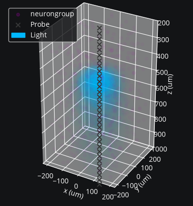
cleo.viz.plot() allows you to easily visualize your experimental configuration:

cleo.viz.plot(ng, colors=['#c500cc'], sim=sim, zlim=(200, 1000))

(<Figure size 640x480 with 1 Axes>,
 <Axes3D: xlabel='x [um]', ylabel='y [um]', zlabel='z [um]'>)

Cleo also features some video visualization capabilities.

Running experiments

Use cleo.CLSimulator.run() function with the desired duration. This wrap’s Brian’s brian2.core.network.Network.run() function:

sim.run(50 * b2.ms)  # kwargs are passed to Brian's run function

Show code cell output Hide code cell output

INFO       No numerical integration method specified for group 'neurongroup', using method 'euler' (took 0.03s, trying other methods took 0.00s). [brian2.stateupdaters.base.method_choice]

INFO       No numerical integration method specified for group 'syn_ChR2_neurongroup', using method 'euler' (took 0.02s, trying other methods took 0.06s). [brian2.stateupdaters.base.method_choice]

Use reset() to restore the default state (right after initialization/injection) for the network and all devices. This could be useful for running a simulation multiple times under different conditions.

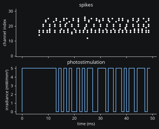
To facilitate access to data after the simulation, devices offer a cleo.InterfaceDevice.save_history option on construction, by default True. If true, that object will store relevant variables as attributes. For example:

import matplotlib.pyplot as plt
fig, (ax1, ax2) = plt.subplots(2, 1, sharex=True)
ax1.scatter(mua.t_ms, mua.i, marker='.', c='white', s=2)
ax1.set(ylabel='channel index', title='spikes')
ax2.step(fiber.t_ms, fiber.values, c='#72b5f2')
ax2.set(xlabel='time (ms)', ylabel='irradiance (mW/mm²)', title='photostimulation')

[Text(0.5, 0, 'time (ms)'),
 Text(0, 0.5, 'irradiance (mW/mm²)'),
 Text(0.5, 1.0, 'photostimulation')]

Design rationale

Why not prototype with more abstract models?

Cleo aims to be practical, and as such provides models at the level of abstraction corresponding to the variables the experimenter has available to manipulate. This means models of spatially defined, spiking neural networks.

Of course, neuroscience is studied at many spatial and temporal scales. While other projects may be better suited for larger segments of the brain and/or longer timescales (such as HNN or BMTK’s PopNet or FilterNet), this project caters to finer-grained models because they can directly simulate the effects of alternate experimental configurations. For example, how would the model change when swapping one opsin for another, using multiple opsins simultaneously, or with heterogeneous expression? How does recording or stimulating one cell type vs. another affect the experiment? Would using a more sophisticated control algorithm be worth the extra compute time, and thus later stimulus delivery, compared to a simpler controller?

Questions like these could be answered using an abstract dynamical system model of a neural circuit, but they would require the extra step of mapping the afore-mentioned details to a suitable abstraction—e.g., estimating a transfer function to model optogenetic stimulation for a given opsin and light configuration. Thus, we haven’t emphasized these sorts of models so far in our development of Cleo, though they should be possible to implement in Brian if you are interested. For example, one could develop a Poisson linear dynamical system (PLDS), record spiking output, and configure stimulation to act directly on the system’s latent state.

And just as experiment prototyping could be done on a more abstract level, it could also be done on an even more realistic level, which we did not deem necessary. That brings us to the next point…

Why Brian?

Brian is a relatively new spiking neural network simulator written in Python. Here are some of its advantages:

• Flexibility: allowing (and requiring!) the user to define models mathematically rather than selecting from a pre-defined library of cell types and features. This enables us to define arbitrary models for recorders and stimulators and easily interface with the simulation

• Ease of use: it’s all just Python

• Speed (at least when compiled to C++ or GPU—see Brian2GENN, Brian2CUDA)

NEST is a popular alternative to Brian also strong in point neuron simulations. However, it appears to be less flexible, and thus harder to extend. NEURON is another popular alternative to Brian. Its main advantage is its first-class support of detailed, morphological, multi-compartment neurons. In fact, strong alternatives to Brian for this project were BioNet (docs, paper) and NetPyNE (docs, paper), which already offer a high-level interface to NEURON with extracellular potential recording. Optogenetics could be incorporated with pre-existing .hoc code, though the light model would need to be implemented. From brief examination of the source code of BioNet, it appears that closed-loop stimulation would not be too difficult to add. It is unclear for NetPyNE.

In the end, we chose Brian since our priority was to model circuit/population-level dynamics over molecular/intra-neuron dynamics. Also, Brian does have support for multi-compartment neurons, albeit less fully featured, if that is needed.

PyNN would have been an ideal interface to build around, as it supports multiple simulator backends. The difficulty is, implementing objects not natively supported by SNN simulators (e.g., opsins, calcium indicators, and light source) has required bespoke, idiosyncratic code applicable only to one simulator. To do so in a native, efficient way, as we have attempted to do with Brian, would require significant work. A collaborative effort extending a multi-simulator framework such as PyNN for this purpose may be of value if there is enough community interest in expanding the open-source SNN experiment simulation toolbox.

Future development

Here are some features which are missing but could be useful to add:

• Electrode microstimulation

• A more accurate LFP signal (only usable for morphological neurons) based on the volume conductor forward model as in LFPy or Vertex

• The Mazzoni-Lindén LFP approximation for LIF point-neuron networks

• Voltage indicators

• An expanded calcium indicator library—currently the parameter set for the full NAOMi model is only available for GCaMP6f. The phenomenological S2F model should be easy to implement and fit to data, has parameters for several of the latest and greatest GECIs (jGCaMP7 and jGCaMP8 varieties), and should be cheaper to simulate as well.